Machine Learning (6) - 关于 Logistic Regression (Multiclass Classification) 的小练习

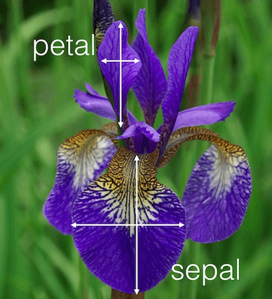
Iris flower data set 是关于一种花的数据集. 这种花有三个品种, 分别是 setosa, virginica 和 versicolor. 每朵花都有两种花瓣(sepals 和 petals).早在 20 世纪 30 年代, 一位学者对每个品种收集了 50 个样本, 分别测量两种花瓣的长度和宽度, 最终形成了一个有 150 条数据的数据集. 这个数据集被广泛用于机器学习的初学者做数据分析的练习.

import pandas as pd
import matplotlib.pyplot as plt
// 引入 iris 数据集
from sklearn.datasets import load_iris
iris = load_iris()

// 查看 iris 数据集的属性
dir(iris)
['DESCR', 'data', 'feature_names', 'filename', 'target', 'target_names']

// 查看 iris 数据集的前5条数据
iris.data[0:5]
// 输出, 分别是每朵花的每种花瓣的长度和宽度
array([[5.1, 3.5, 1.4, 0.2],
       [4.9, 3. , 1.4, 0.2],
       [4.7, 3.2, 1.3, 0.2],
       [4.6, 3.1, 1.5, 0.2],
       [5. , 3.6, 1.4, 0.2]])

// 查看 iris 数据集的属性名称
iris.feature_names
// 输出
['sepal length (cm)',
 'sepal width (cm)',
 'petal length (cm)',
 'petal width (cm)']

iris.target
// 输出
array([0, 0, 0, 0, 0, 0, 0, 0, 0, 0, 0, 0, 0, 0, 0, 0, 0, 0, 0, 0, 0, 0,
       0, 0, 0, 0, 0, 0, 0, 0, 0, 0, 0, 0, 0, 0, 0, 0, 0, 0, 0, 0, 0, 0,
       0, 0, 0, 0, 0, 0, 1, 1, 1, 1, 1, 1, 1, 1, 1, 1, 1, 1, 1, 1, 1, 1,
       1, 1, 1, 1, 1, 1, 1, 1, 1, 1, 1, 1, 1, 1, 1, 1, 1, 1, 1, 1, 1, 1,
       1, 1, 1, 1, 1, 1, 1, 1, 1, 1, 1, 1, 2, 2, 2, 2, 2, 2, 2, 2, 2, 2,
       2, 2, 2, 2, 2, 2, 2, 2, 2, 2, 2, 2, 2, 2, 2, 2, 2, 2, 2, 2, 2, 2,
       2, 2, 2, 2, 2, 2, 2, 2, 2, 2, 2, 2, 2, 2, 2, 2, 2, 2])

// 这里就是 iris 花的三个品种的名字, 应该是分别对应了 target 值的 0, 1, 2
iris.target_names
//输出
array(['setosa', 'versicolor', 'virginica'], dtype='<U10')

// 把数据集拆分为训练数据和测试数据
from sklearn.model_selection import train_test_split
X_train, X_test, y_train, y_test = train_test_split(iris.data, iris.target, test_size=0.2)
len(X_train) // 120
len(X_test) // 30

// 训练模型
from sklearn.linear_model import LogisticRegression
model = LogisticRegression()
model.fit(X_train, y_train)

// 查看模型准确度
model.score(X_test, y_test) // 0.9

// 通过模型进行预测
model.predict([[4.4, 3., 1.6, 0.9]])
// 输出
array([0])

想要更加细致地了解误差的位置, 可以通过 confusion_matrix 类实现:

// 通过模型预测的值
y_predicted = model.predict(X_test)

// 引入 confusion_matrix 包
from sklearn.metrics import confusion_matrix
cm = confusion_matrix(y_test, y_predicted)
cm
// 输出
array([[ 7,  0,  0],
       [ 0,  8,  2],
       [ 0,  0, 13]])

// 为了将上面的输出可视化更强, 引入 seaborn 包     
import seaborn as sn
plt.figure(figsize = (10, 7))
sn.heatmap(cm, annot=True)
plt.xlabel('Predicted')
plt.ylabel('Truth')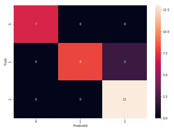

本作品采用《CC 协议》，转载必须注明作者和本文链接