
003.00 监督式学习
0 / 0 / 创建于 6年前 /
 Jason990420 的个人博客
003.00 监督式学习
建檔日期: 2019/09/17
更新日期: None
相关软件信息:
| Win 10 | Python 3.7.2 |
说明:所有内容欢迎引用,只需注明来源及作者,本文内容如有错误或用词不当,敬请指正.
主题: 003.00 监督式学习
前言:
看到人工智能, 机器学习, 再到深度学习, 一大堆杂七杂八的数据, 得花多久的时间才能搞懂作什么, 先找了一个范例, 这个范例是采用100张的明星照片, 建立一个模型用来分辨照片中的明星是男是女, 先区分为80张的训练组及20张的测试组, 除了图片以外, 还要自行确认每张照片中的明星是男是女, 建立性别数据. 该模型输出只有两种类别, 男或女, 或者说是不是男的, 或者说是不是女的, 这是一种二选一分类的模型, 不同的功能会有不同的模型, 这里采用的是逻辑回归的算法.
本范例主要的是采用numpy来作所有的处理, 而不是如其的人工智能库给你一个函数, 什么都作完了, 这样你不会清楚知道发生什么事. 在本范例中了解了整个模型建构及算法细节, 感觉在人工智能上跨了一大步.
范例来源: https://datascienceintuition.wordpress.com...
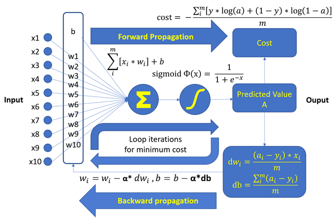
要一步一步的说明细节, 不如看下图比较直接, 后面再稍作解释, 就容易看懂了.
1. 准备数据作为输入
a. 照片来源
照片当然可以自己拍, 不过挺花时间的, 在学习阶段, 直接上网下载就行, 网上有很多数据库免费提供, 比如: https://lionbridge.ai/datasets/the-50-best....
一般的库大都是一行就下载下来, 这里是从网页中读取100张的照片, 存放到子目录中, 下次就不用再下载一次
def load_100_pictures():
    if not os.path.exists('img_align_celeba'):
        os.mkdir('img_align_celeba')
        for img_i in range(1, 101):
            f = '000%03d.jpg' % img_i
            url = 'https://s3.amazonaws.com/cadl/celeb-align/' + f
            print(url, end='\r')
            urllib.request.urlretrieve(url, os.path.join('img_align_celeba', f))
    print('Celeb Net dataset already downloaded')
b. 资料分为两群, 训练群及测试群.
一般测试群大约占1/4数据, 这个比例可以自行分配. 训练群用来让模型找到自己内部最佳的参数, 也就是wi及b. 测试群用来测试最后模型的准确性.
c. 照片为jpg檔
每一个像素都含有三个0~255的R,G,B值, 光的三要素R(红),G(绿),B(蓝)合成在一起, 才是该像素的颜色.
d. 照片资料的shape为(100张, 218高, 178寛, 3色)
在输入到模型中, 必须先处理一下, 才能符合模型的输入要求. 除了简单化, 也可以减少内存的使用和处理的时间. 不过, 过度的简化可能会造成信息量的流失, 造成模型建造失败.
e. 每张照片高218像素, 寛178像素
我们先裁成(178, 178)的正方形. 照片群就变成(100张, 178高, 178寛, 3色), 数据量一下就少了20%左右.
def imcrop_tosquare(img):
    if img.shape[0] > img.shape[1]:
        extra = (img.shape[0] - img.shape[1]) // 2
        crop = img[extra:-extra, :]
    elif img.shape[1] > img.shape[0]:
        extra = (img.shape[1] - img.shape[0]) // 2
        crop = img[:, extra:-extra]
    else:
        crop = img
    return crop
f. 将照片的尺寸由(178, 178)改为(64, 64)
缩小的照小在人眼看来, 仍然可以轻易辨认出性别来. 照片群就变成(100张, 64高, 64寛, 3色), 因为这个尺寸是以平方来计算的, 所以数据量一下就少了87%左右, 总计数据量只有约原来的10%. 当然, 我们还可以再把RGB三色转换为灰阶, 数据量就会变成只有约原来的3.3%, 不过我们还是保留没有这样作, 当然各位可以试试.
imgs = []
for file_i in files:
    # 照片格式都是(218, 178, 3), 高218, 寛178, RGB三色/每点
    img = plt.imread(file_i)
    # 裁成(178,178,3), 正方形照片
    square = imcrop_tosquare(img)
    # 以LANCZOS方法来重设大小为(64,64,3),
    # 足以辨识就可以了, 照片太大, 处理时间与内存都会占用太多
    rsz = np.array(Image.fromarray(square).resize((64, 64), resample=Image.LANCZOS))
    # list结果为(100, 64, 64, 3), 100笔, 64x64, RGB三色的照片资料
    imgs.append(rsz)
g. 再把数据从 0 ~ 255 转为 0 ~ 1
在逻辑回归計算时, 有使用到指数的运算, 大于1的数, 很容易就会造成系统数值溢出错误.
data = np.array(imgs)/255h. 建立資料标签
照片资料中并没有我们所要的性别数据, 所以我们要自己看照片判断建立. 还有建立两个分类的标签[‘Male 男’, ‘Female 女’], 这里我们定义0为男性, 1为女性.
classes=np.array(['Male', 'Female'])
y=np.array([1,1,0,1,1,1,0,0,1,1,1,0,0,1,0,0,1,1,1,0,0,1,0,1,0,1,1,1,1,0,1,0,0,1,1,0,0,0,1,1,0,1,1,1,1,1,1,0,0,0,0,0,0,1,0,0,1,1,1,0,0,1,1,0,0,1,0,0,0,0,1,0,1,1,1,0,1,1,0,0,0,0,1,1,1,1,1,1,1,0,0,1,1,1,1,1,1,1,1,1])
y=y.reshape(1,y.shape[0])
i. 把照片分为两群, 训练群及测试群
train_x_orig=data[:80,:,:,:]
test_x_orig=data[80:,:,:,:]
y_train=y[:,:80]
y_test=y[:,80:]
j. 最后我们要把二维的像素数据转换为一维的像素数据
这样才能符合模型的输入要求. 转换的方式是把每一行的点连续接在一起再转置, 如此一来, 训练组照片从(80, 64, 64, 3)变为(12288,80), 测试组照片从(20,64,64,3)变为(12288,20).
# 训练数据80笔, 测试资料20笔, 照片每边64点
m_train = train_x_orig.shape[0]
m_test = y_test.shape[1]
num_px = train_x_orig.shape[1]
# (80, 64, 64, 3) -> (1228,80), (20,64,64,3) -> (1228,20)
train_x = train_x_orig.reshape(train_x_orig.shape[0],-1).T
test_x = test_x_orig.reshape(test_x_orig.shape[0],-1).T
2. 对每一笔输入训练用数据的特征值X或xi随意设置权重W或wi, 并随意设置一个偏差值b
在这里, 简单为主, 我们都设为0
    w = np.zeros((1,12288))
    b = 0
3. 计算sigma, Σ值
只要在计算前把矩阵的shape, 也就是数据摆对方向及位置, 就会很容易计算, 这也是numpy数组强大的所在, 简单的一个运算就把事情作完了.
sigma =np.dot(w,X)+b4. 使用sigmoid函数
将Σ作非线性转换成-1 ~ 1的数值, 得到我们的预测值A或a, A中的每一项a就代表该照片经模型预测的性别结果, 因为在模型中, 利用预测A与实际Y的差异去调整权重wi及偏差b, 以得到更接近实际Y的预测A, 这也是负回馈的一种应用.
def sigmoid(z):
    # 建立sigmoid函数, 将输入值非线性转换为-1~+1的数值
    s = 1/(1+np.exp(-z))
    return s
A = sigmoid(np.dot(w,X)+b)
5. 以逻辑回归的方式, 计算误差值
这里称为成本cost, 原则上, cost越小越好, 因为cost可以代表所有预测值与实际值的差异或误差值总和.
cost = (-1/m)*(np.dot(Y,np.log(A.T))+ np.dot((1-Y),np.log((1-A).T)))6. 根据输入的特征值, 预测值及测试用的实际值, 计算成本对权重wi的导数dw (实际上是dcost/dw), 以及对偏差值b的导数db (实际上是dcost/db)
在sigma Σ中, xi不是一个变量, 是已知的输入数据, wi及b才是在模型作训练时的变量, 所以我们要对wi及b来求导数, 用来作为回归方法中的反馈参数. 导数代表的意义是指该变量的变化量, 所造成输出的变化量, 导数值越大, 变化量越大, 我们要调整wi或b的量就越大, 越接近最低点, 导数值就越小, 一直到导数值为0, 或足够接近0, 最低点的导数或斜率就是0.
    dw = (1/m)*np.dot((A-Y),X.T)
    db = (1/m)*np.sum((A-Y))
7. 根据成本对权重wi的导数,对偏差值b的导数, 以及alpha或α, 修改wi及b
这里的alpha或α, 用来对调整的量作一个限制, 因为调整太多, 会找不到最低点, 调整太少会花太多的时间在调整上, 所以alpha或α被称为学习速率. 一般来说, alpha值大都在1以下, 当然也有使用1以上的情况, 甚至可能是上千. 这个值的设置是随情况而定的, 也可以说是试出来的.
        w = w-learning_rate*dw
        b = b-learning_rate*db
8. 重复N次步骤3到步骤7, 得到最小的cost, 最适当的wi及b值.
N是模型更新wi及b的次数, 多少次才是对的, 这是不一定的, 因为要看模型的复杂度, alpha值的选择, 通常有个上限, 因为作得再多次, 结果变化也不大. 模型中所用的方法是数值分析的一种, 基本上, 作的更多次, 会更靠近目标点, 只是更靠近, 并不一定会落在目标点上. 简单的模型, 可能很快就可以找到目标点, 但在复杂的模型中, 作得太多次可能会更糟糕, 这种情形就叫作over-fitting过度拟合或过适, 因为这里追求的是训练组的磨合, 结果可能测试组的结果变差了, 而我们真正要的结果是测试组的结果.
9. 使用该模型, 根据已知最适当的wi及b值, 计算出训练组数据的预测值
与实际值作比较, 确认训练后的正确率是否够好, 不够好可以调整alpha值及N值, 也有可能是该模型的建构方式无法符合要求, 必须采用不同的模型来重新训练及测试.
10. 使用该模型, 根据已知最适当的wi及b值, 计算出测试组数据的预测值
与实际值作比较, 确认训练后, 该模型的正确率是否够好, 是否可以适用到一般的应用上.
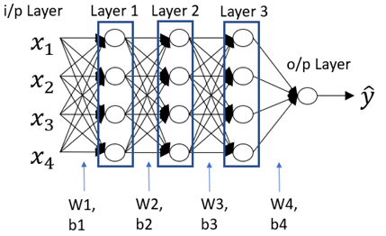
结论: 本文所述的模型因为简单, 所以在输入层与输出层中, 只有一层的wi及b, 所计算出来的训练组正确率达到100%, 但测试组的正确率却只有65%, 可以有很多的方式来改善, 比如:
- 这里用的梯度下降法是最常用的方法, 但只能在简单的模型中找到目标点; 在复杂的模型中可能只是找到局部的目标点, 而不是全局的目标点.
- 使用更多层的wi和b, 这代表更复杂的模型, 在很多人工智能的建模都可以看到, 如下图.
- 数据量的保留, 缩减通常会造成信息的流失
- 改变不同的算法, 比如模型中的sigma Σ, sigmoid, cost, 回归法等等
输出结果:
运算次数与cost的对照表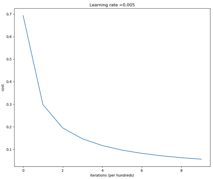
测试组中预测错误的七张照片
原照片与经加权/偏移计算的照片比对
附件(程序)
# -*- coding: utf-8 -*-
import os
import urllib.request
import numpy as np
import matplotlib.pyplot as plt
from PIL import Image

def load_100_pictures():
    if not os.path.exists('img_align_celeba'):
        os.mkdir('img_align_celeba')
        for img_i in range(1, 101):
            f = '000%03d.jpg' % img_i
            url = 'https://s3.amazonaws.com/cadl/celeb-align/' + f
            print(url, end='\r')
            urllib.request.urlretrieve(url, os.path.join('img_align_celeba', f))
    print('Celeb Net dataset already downloaded')

# 从网站下载100张明星照片, 在到img_align_celeba目录下, 如果目录已存在, 就不下载了
load_100_pictures()
# 从目录中取得所有JPG文件的档名(长度100的list)
files = [os.path.join('img_align_celeba', file_i) for file_i in os.listdir('img_align_celeba') if '.jpg' in file_i]

# 自行建立一个数组, 内容为各照片中明星的性别, 0为男性, 1为女性
# shape从(100,)改为(1,100)
y=np.array([1,1,0,1,1,1,0,0,1,1,1,0,0,1,0,0,1,1,1,0,0,1,0,1,0,1,1,1,1,0,1,0,0,1,1,0,0,0,1,1,0,1,1,1,1,1,1,0,0,0,0,0,0,1,0,0,1,1,1,0,0,1,1,0,0,1,0,0,0,0,1,0,1,1,1,0,1,1,0,0,0,0,1,1,1,1,1,1,1,0,0,1,1,1,1,1,1,1,1,1])
y=y.reshape(1,y.shape[0])

# 建立分类标签内容'Male', 'Female'
classes=np.array(['Male', 'Female'])

# 目标分为两群, 前80张为训练用群, 后20张为测试群
y_train=y[:,:80]
y_test=y[:,80:]

# 截取照片成最大的正方形
def imcrop_tosquare(img):
    if img.shape[0] > img.shape[1]:
        extra = (img.shape[0] - img.shape[1]) // 2
        crop = img[extra:-extra, :]
    elif img.shape[1] > img.shape[0]:
        extra = (img.shape[1] - img.shape[0]) // 2
        crop = img[:, extra:-extra]
    else:
        crop = img
    return crop

# 读入所有的照片
imgs = []
for file_i in files:
    # 照片格式都是(218, 178, 3), 高218, 寛178, RGB三色/每点
    img = plt.imread(file_i)
    # 裁成(178,178,3), 正方形照片
    square = imcrop_tosquare(img)
    # 以LANCZOS方法来重设大小为(64,64,3),
    # 足以辨识就可以了, 照片太大, 处理时间与内存都会占用太多
    rsz = np.array(Image.fromarray(square).resize((64, 64), resample=Image.LANCZOS))
    # list结果为(100, 64, 64, 3), 100笔, 64x64, RGB三色的照片资料
    imgs.append(rsz)

# 降低数据大小, 避免在逻辑回归时, 指数运算造成系统数值溢出错误
data = np.array(imgs)/255

# 资料分为两群, 前80张为训练用群, 后20张为测试群
train_x_orig=data[:80,:,:,:]
test_x_orig=data[80:,:,:,:]

# 对只有两种结果的事件, 采用逻辑回归法

# 训练数据80笔, 测试资料20笔, 照片每边64点
m_train = train_x_orig.shape[0]
m_test = y_test.shape[1]
num_px = train_x_orig.shape[1]

# (80, 64, 64, 3) -> (12288,80), (20,64,64,3) -> (12288,20)
train_x = train_x_orig.reshape(train_x_orig.shape[0],-1).T
test_x = test_x_orig.reshape(test_x_orig.shape[0],-1).T

# Initialize parameters W and b

def initialize_with_zeros(dim):
    # 建立w是一个内容都为0, 点数大小的数组(1, 点数12288), b为0
    w = np.zeros((1,dim))
    b = 0
    # 确认w及b符合要求
    assert(w.shape == (1, dim))
    assert(isinstance(b, float) or isinstance(b, int))
    return w, b

def sigmoid(z):
    # 建立sigmoid函数, 将输入值非线性转换为-1~+1的数值
    s = 1/(1+np.exp(-z))
    return s

def propagate(w, b, X, Y):
    '''
    输入
    w -- 加权数组, 对应到一张照片所有的点的三颜色, (点数*3, 1) (12288, 1)
    b -- 偏差, 纯量
    X -- 输入的数据数组, (点数*3, 训练用照片数) (12288, 80)
    Y -- 结果卷标0, 1的数组, (1, 训练用照片数) (1, 80)

    输出:
    cost -- 负对数可能值, 是逻辑回归法中的成本或误差值
    dw -- dcost/dw, (点数*3, 1)
    db -- dcost/db, 纯量

    '''
    m = X.shape[1]
    # 正向传递 (从输入到成本 X -> cost), A预测值(1, 80), cost = -1/m*sum(y*log(a)+(1-y)*log(1-a)
    A = sigmoid(np.dot(w,X)+b)
    cost = (-1/m)*(np.dot(Y,np.log(A.T))+ np.dot((1-Y),np.log((1-A).T)))
    # 反向传递 (找出梯度grads), dZ=A-Y, dw = 1/m*(dZ . XT), db = mean(dZ)
    dw = (1/m)*np.dot((A-Y),X.T)
    db = (1/m)*np.sum((A-Y))
    assert(dw.shape == w.shape)
    assert(db.dtype == float)
    cost = np.squeeze(cost)
    assert(cost.shape == ())
    grads = {"dw": dw,
             "db": db}
    return grads, cost

def optimize(w, b, X, Y, num_iterations, learning_rate, print_cost = False):
    """
    利用梯度下降算法优化 w, b

    输入
    w -- 加权数组, 对应到一张照片所有的点的三颜色, (点数*3, 1) (12288, 1)
    b -- 偏差, 纯量
    X -- 所有输入的数据数组, (点数*3, 训练用照片数) (12288, 80)
    Y -- 结果卷标0, 1的数组, (1, 训练用照片数) (1, 80)
    num_iterations -- 参数优化运算次数
    learning_rate -- 参数修正学习速率
    print_cost -- 是否每100次运算, 打印成本cost

    输出
    params -- { } w, b
    grads -- {'dw':dw, 'db':db'} cost对w的导数, cost对b的导数
    costs -- [ ] 所有cost记录, 供画图使用

    """

    costs = []

    for i in range(num_iterations):

        # 按输入数据, 目标卷标, 模型中的权重及偏移值计算成本Cost及梯度
        grads, cost = propagate(w, b, X, Y)

        # 从grads中取回dw, db
        dw = grads["dw"]
        db = grads["db"]

        # 更新权重及偏差
        w = w-learning_rate*dw
        b = b-learning_rate*db

        # 每100次记录下cost值
        if i % 100 == 0:
            costs.append(cost)

        # 是否每100次打印cost
        if print_cost and i % 100 == 0:
            print ("Cost after iteration %i: %f" %(i, cost))

    # 画cost曲线
    plt.rcParams['figure.figsize'] = (10.0, 10.0)
    plt.plot(np.squeeze(costs))
    plt.ylabel('cost')
    plt.xlabel('iterations (per hundreds)')
    plt.title("Learning rate =" + str(learning_rate))
    plt.show()
    params = {"w": w, "b": b}
    grads = {"dw": dw, "db": db}

    return params, grads, costs

def predict(w, b, X):
    '''
    按已优化的 w, b 预测输入的照片结果

    输入
    w -- 模型中已优化的权重 (12288, 1)
    b -- 偏差值
    X -- 输入料数组 (12288, 照片数)

    输出
    Y_prediction -- 预测结果
    '''

    m = X.shape[1]
    Y_prediction = np.zeros((1,m))
    #w = w.reshape(X.shape[0], 1)

    # 计算预测值, 并转成0~1的机率值, 再四舍五入取整数
    A = sigmoid(np.dot(w,X)+b)
    Y_prediction=np.round(A)

    assert(Y_prediction.shape == (1, m))

    return Y_prediction

def model(X_train, Y_train, X_test, Y_test, num_iterations = 2000, learning_rate = 0.5, print_cost = False):
    """
    建立逻辑回归模型

    输入参数
    X_train -- 训练用输入的数据数组, (点数*3, 训练用照片数) (12288, 80)
    Y_train -- 训练用结果卷标0, 1的数组, (1, 训练用照片数) (1, 80)
    X_test -- 测试用输入的数据数组, (点数*3, 测试用照片数) (12288, 20)
    Y_test -- 测试用结果卷标0, 1的数组, (1, 训练用照片数) (1, 20)
    num_iterations -- 参数优化运算次数
    learning_rate -- 参数修正学习速率
    print_cost -- 是否每100次运算, 打印成本cost

    输出:
    d -- { } 有关模型的信息
    """

    # 初值选定 (1, 12288)
    m_train=X_train.shape[0]
    w, b = initialize_with_zeros(m_train)

    # 梯度下降优化
    parameters, grads, costs = optimize(w, b, X_train, Y_train, num_iterations= num_iterations, learning_rate = learning_rate, print_cost = print_cost)

    # 取出 w, b
    w = parameters["w"]
    b = parameters["b"]

    # 检查训练组及测试组
    Y_prediction_test = predict(w, b, X_test)
    Y_prediction_train = predict(w, b, X_train)

    # 打印检查正确率
    print("train accuracy: {} %".format(100*(1 - np.mean(np.abs(Y_prediction_train - Y_train)) )))
    print("test accuracy: {} %".format(100*(1 - np.mean(np.abs(Y_prediction_test - Y_test)) )))

    d = {"costs": costs,
         "Y_prediction_test": Y_prediction_test,
         "Y_prediction_train" : Y_prediction_train,
         "w" : w,
         "b" : b,
         "learning_rate" : learning_rate,
         "num_iterations": num_iterations}

    return d

d = model(train_x, y_train, test_x, y_test, num_iterations = 1000, learning_rate = 0.005, print_cost = True)

def print_mislabeled_images(classes, X, y, p):
    """
    显示在测试组判断错误的照片
    X -- 照片资料组
    y -- 正确标签组
    p -- 预测标签组
    """
    a = p + y
    mislabeled_indices = np.asarray(np.where(a == 1))
    plt.rcParams['figure.figsize'] = (40.0, 40.0) # set default size of plots
    num_images = len(mislabeled_indices[0])
    for i in range(num_images):
        index = mislabeled_indices[1][i]

        plt.subplot(2, num_images, i + 1)
        plt.imshow(X[:,index].reshape(64,64,3), interpolation='sinc')
        plt.axis('off')
        plt.rc('font', size=10)
        plt.title("Prediction: " + classes[int(p[0,index])] + " \n Class: " + classes[y[0,index]])
    plt.show()

print_mislabeled_images(classes, test_x, y_test, d["Y_prediction_test"])

# 使用sinc函数来重建经过比重后的照片

test=d["w"].T*train_x*255
test=test.T.reshape(80,64,64,3)
plt.rcParams['figure.figsize'] = (10.0, 10.0)
plt.imshow(test[0], interpolation='sinc')

# reconstructed data by others

methods = [None, 'none', 'nearest', 'bilinear', 'bicubic', 'spline16',
           'spline36', 'hanning', 'hamming', 'hermite', 'kaiser', 'quadric',
           'catrom', 'gaussian', 'bessel', 'mitchell', 'sinc', 'lanczos']

# Fixing random state for reproducibility
np.random.seed(19680801)

fig, axes = plt.subplots(3, 6, figsize=(24, 12),
                         subplot_kw={'xticks': [], 'yticks': []})

fig.subplots_adjust(hspace=0.3, wspace=0.05)

for ax, interp_method in zip(axes.flat, methods):
    ax.imshow(test[0], interpolation=interp_method, cmap=None)
    ax.set_title(interp_method)

plt.show()

# compare the reconstructed images vs original.

def montage(images, saveto='montage.png'):
    """Draw all images as a montage separated by 1 pixel borders.
    Also saves the file to the destination specified by `saveto`.
    Parameters
    ----------
    images : numpy.ndarray
        Input array to create montage of.  Array should be:
        batch x height x width x channels.
    saveto : str
        Location to save the resulting montage image.
    Returns
    -------
    m : numpy.ndarray
        Montage image.
    """
    if isinstance(images, list):
        images = np.array(images)
    img_h = images.shape[1]
    img_w = images.shape[2]
    n_plots = int(np.ceil(np.sqrt(images.shape[0])))
    if len(images.shape) == 4 and images.shape[3] == 3:
        m = np.ones(
            (images.shape[1] * n_plots + n_plots + 1,
             images.shape[2] * n_plots + n_plots + 1, 3)) * 0.5
    else:
        m = np.ones(
            (images.shape[1] * n_plots + n_plots + 1,
             images.shape[2] * n_plots + n_plots + 1)) * 0.5
    for i in range(n_plots):
        for j in range(n_plots):
            this_filter = i * n_plots + j
            if this_filter < images.shape[0]:
                this_img = images[this_filter]
                m[1 + i + i * img_h:1 + i + (i + 1) * img_h,
                  1 + j + j * img_w:1 + j + (j + 1) * img_w] = this_img
    #plt.imsave(arr=m, fname=saveto)
    return m

compare = np.concatenate((test[52:54], data[52:54]), axis=0)
compare.shape

plt.imshow(montage(compare,saveto='montage.png'),interpolation='spline36')
plt.show()
plt.imshow(montage(compare,saveto='montage.png'),interpolation='bicubic')
plt.show()

# generate the montage with different interpolations for comparison.

methods = [None, 'none', 'nearest', 'bilinear', 'bicubic', 'spline16',
           'spline36', 'hanning', 'hamming', 'hermite', 'kaiser', 'quadric',
           'catrom', 'gaussian', 'bessel', 'mitchell', 'sinc', 'lanczos']

# Fixing random state for reproducibility
np.random.seed(19680801)

fig, axes = plt.subplots(3, 6, figsize=(24, 12),
                         subplot_kw={'xticks': [], 'yticks': []})

fig.subplots_adjust(hspace=0.3, wspace=0.05)

for ax, interp_method in zip(axes.flat, methods):
    ax.imshow(montage(compare,saveto='montage.png'), interpolation=interp_method, cmap=None)
    ax.set_title(interp_method)

plt.show()本作品采用《CC 协议》,转载必须注明作者和本文链接


 关于 LearnKu


推荐文章: