查看 librosa 版本

import librosa
print(librosa.__version__)

y 为信号向量。
sr 为采样率。
y[1000] 表示信号的第 1001 个样本。
S[:,100] 表示 S 的第 101 帧。
默认参数：sr = 22050，hop_length = 512。

librosa.core

• Low-level audio processes（低级音频处理）
• Unit conversion（单位换算）
• Time-frequency representations（时频表示）

要以其原始采样率家在信号，使用 sr=None。
To load a signal at its native sampling rate, use sr=None

y_orig, sr_orig = librosa.load(librosa.util.example_audio_file(),
                     sr=None)
print(len(y_orig), sr_orig)

[Out]: 2710336 44100

Resampling is easy

sr = 22050
y = librosa.resample(y_orig, sr_orig, sr)
print(len(y), sr)

[Out]: 1355168 22050

But what’s that in seconds?

print(librosa.samples_to_time(len(y), sr))

[Out]: 61 .45886621315193

Spectral representations

Short-time Fourier transform underlies most analysis.
短时傅立叶变换是大多数分析的基础。
librosa.stft returns a complex matrix D.
librosa.stft 返回一个复数矩阵 D。
D[f, t] is the FFT value at frequency f, time (frame) t.
D[f, t] 是在频率 f，时间（帧）处的 FFT 值 t。

D = librosa.stft(y)
print(D.shape, D.dtype)

[Out]: (1025, 2647) complex64

Often, we only care about the magnitude.
通常，我们只关心幅度。
D contains both magnitude S and phase 𝜙.
D 包含幅度 S 和相位 𝜙。

D_{ft}=S_{ft}\exp(j\phi_{ft})

import numpy as np

S, phase = librosa.magphase(D)
print(S.dtype, phase.dtype, np.allclose(D, S * phase))

[Out]: float32 complex64 True

Constant-Q transforms

The CQT gives a logarithmically spaced frequency basis.
CQT提供了对数间隔的频率基础。
This representation is more natural for many analysis tasks.
对于许多分析任务而言，这种表示更为自然。

C = librosa.cqt(y, sr=sr)
print(C.shape, C.dtype)

[Out]: (84, 2647) complex128

Exercise 0

• Load a different audio file
• Compute its STFT with a different hop length

# Exercise 0 solution
y2, sr2 = librosa.load(   )
D = librosa.stft(y2, hop_length=   )

librosa.feature

• Standard features(标准功能):
  • librosa.feature.melspectrogram
  • librosa.feature.mfcc
  • librosa.feature.chroma
  • Lots more…
• Feature manipulation(功能操纵):
  • librosa.feature.stack_memory
  • librosa.feature.delta

大多数功能都可与音频或 STFT 输入配合使用
Most features work either with audio or STFT input

melspec = librosa.feature.melspectrogram(y=y, sr=sr)
# Melspec assumes power, not energy as input
# 假定功率作为输入, 而非能量
melspec_stft = librosa.feature.melspectrogram(S=S**2, sr=sr)
print(np.allclose(melspec, melspec_stft))

Out: True

librosa.display

• Plotting routines for spectra and waveforms
  频谱和波形的绘图例程
• Note: major overhaul coming in 0.5

# Displays are built with matplotlib 
import matplotlib.pyplot as plt

# Let's make plots pretty
import matplotlib.style as ms
ms.use('seaborn-muted')

# Render figures interactively in the notebook
%matplotlib nbagg

# IPython gives us an audio widget for playback
from IPython.display import Audio

import librosa.display

Waveform display

plt.figure()
librosa.display.waveplot(y=y, sr=sr)

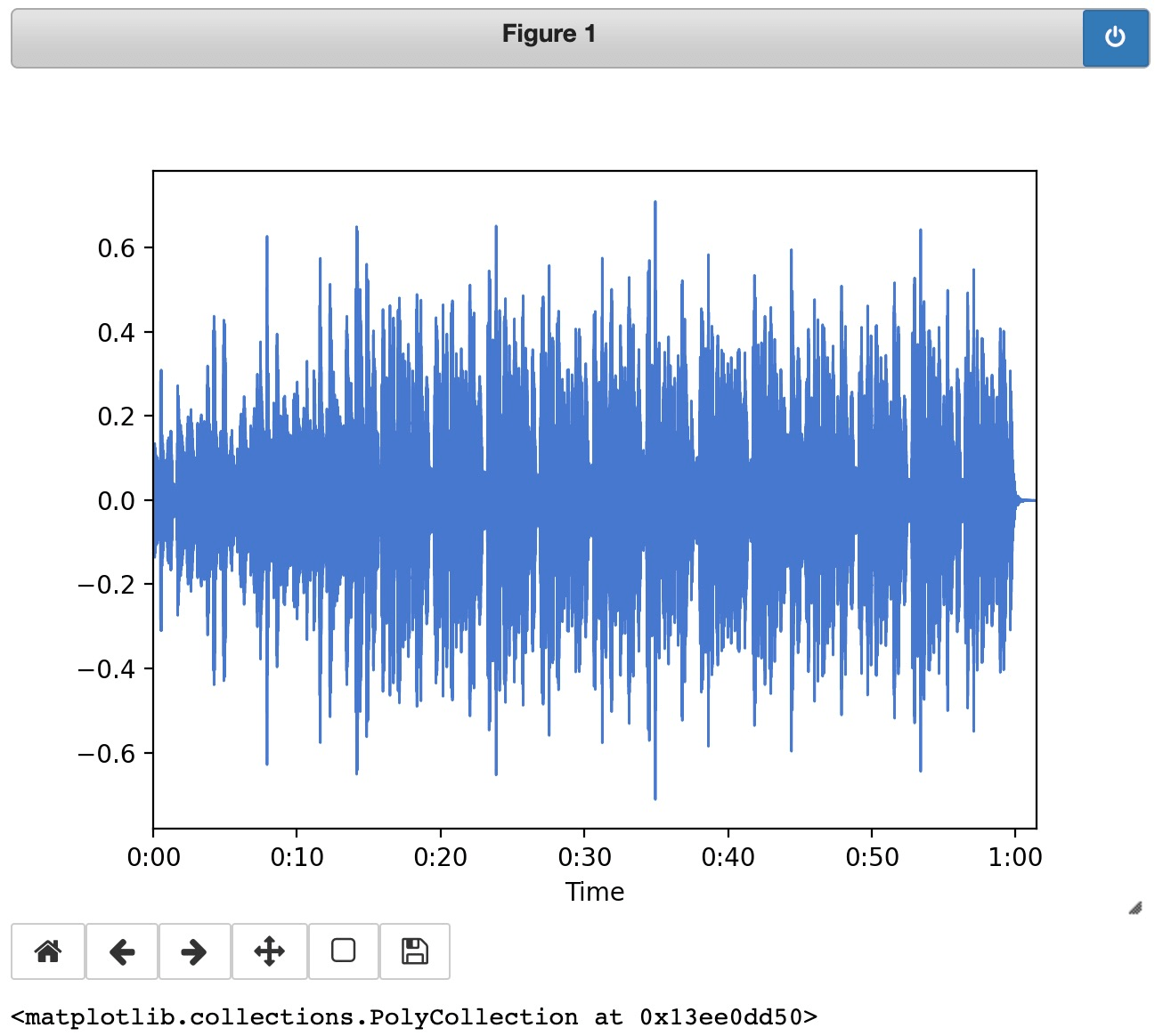
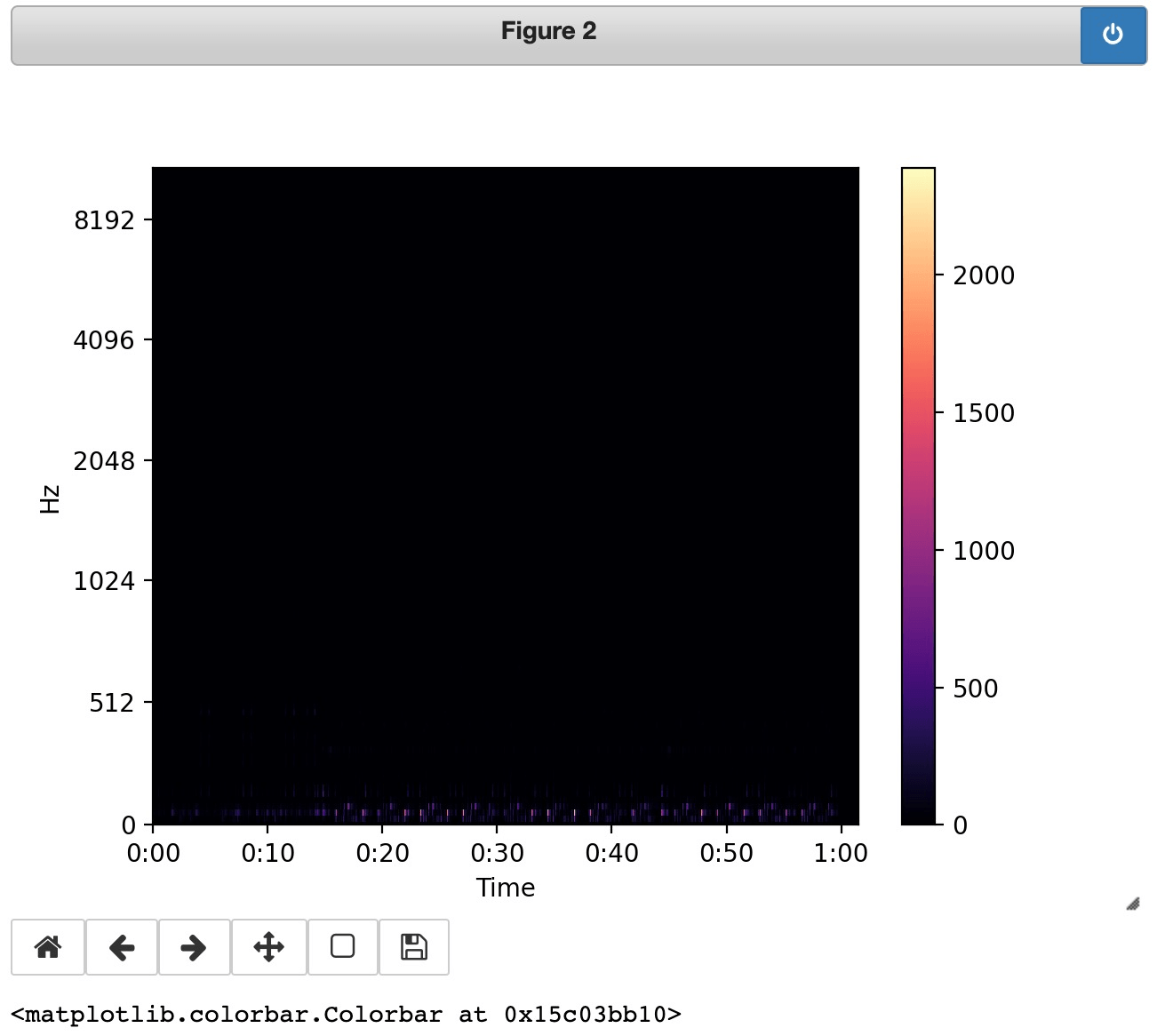
A basic spectrogram display

plt.figure()
librosa.display.specshow(melspec, y_axis='mel', x_axis='time')
plt.colorbar()

Exercise 1

• Pick a feature extractor from the librosa.feature submodule and plot the output with librosa.display.specshow

• Bonus: Customize the plot using either specshow arguments or pyplot functions

# Exercise 1 solution

X = librosa.feature.XX()

plt.figure()

librosa.display.specshow(    )

librosa.beat

• Beat tracking and tempo estimation
  节拍跟踪和速度估计

The beat tracker returns the estimated tempo and beat positions (measured in frames)
节拍跟踪器返回估计的速度和节拍位置（以帧为单位）

tempo, beats = librosa.beat.beat_track(y=y, sr=sr)
print(tempo)
print(beats)

[Out]: 129 .19921875
[ 5 24 43 63 83 103 122 142 162 182 202 222 242 262
281 301 321 341 361 382 401 421 441 461 480 500 520 540
560 580 600 620 639 658 678 698 718 737 758 777 798 817
837 857 877 896 917 936 957 976 996 1016 1036 1055 1075 1095
1116 1135 1155 1175 1195 1214 1234 1254 1275 1295 1315 1334 1354 1373
1394 1414 1434 1453 1473 1493 1513 1532 1553 1573 1593 1612 1632 1652
1672 1691 1712 1732 1752 1771 1791 1811 1831 1850 1871 1890 1911 1931
1951 1971 1990 2010 2030 2050 2070 2090 2110 2130 2150 2170 2190 2209
2229 2249 2269 2289 2309 2328 2348 2368 2388 2408 2428 2448 2468 2488
2508 2527 2547]

Let’s sonify it!

clicks = librosa.clicks(frames=beats, sr=sr, length=len(y))

Audio(data=y + clicks, rate=sr)

Beats can be used to downsample features

chroma = librosa.feature.chroma_cqt(y=y, sr=sr)
chroma_sync = librosa.feature.sync(chroma, beats)

AttributeError: module ‘librosa.feature’ has no attribute ‘sync’
留意下，新版本的 librosa.feature 里没有 ‘sync’ 属性了。

plt.figure(figsize=(6, 3))
plt.subplot(2, 1, 1)
librosa.display.specshow(chroma, y_axis='chroma')
plt.ylabel('Full resolution')
plt.subplot(2, 1, 2)
librosa.display.specshow(chroma_sync, y_axis='chroma')
plt.ylabel('Beat sync')

NameError: name ‘chroma_sync’ is not defined

librosa.segment

• Self-similarity / recurrence
  自相关 / 重现
• Segmentation
  分割

Recurrence matrices encode self-similarity
递归矩阵编码自相关

R[i, j] = similarity between frames (i, j)

Librosa computes recurrence between k-nearest neighbors.

Librosa 计算 k -nearest 邻居之间的递归。

R = librosa.segment.recurrence_matrix(chroma_sync)

plt.figure(figsize=(4, 4))
librosa.display.specshow(R)

We can include affinity weights for each link as well.
我们还可以引入每个链接的关系权重。

R2 = librosa.segment.recurrence_matrix(chroma_sync, mode='affinity', sym=True)

plt.figure(figsize=(5, 4))
librosa.display.specshow(R2)
plt.colorbar()

Exercise 2

• Plot a recurrence matrix using different features
• Bonus: Use a custom distance metric

# Exercise 2 solution

librosa.decompose

• hpss: Harmonic-percussive source separation
• nn_filter: Nearest-neighbor filtering, non-local means, Repet-SIM
• decompose: NMF, PCA and friends

Separating harmonics from percussives is easy
将谐波与打击乐分开很容易

D_harm, D_perc = librosa.decompose.hpss(D)
y_harm = librosa.istft(D_harm)
y_perc = librosa.istft(D_perc)

然后可以自己听一下分开后的音乐

Audio(data=y_harm, rate=sr)
Audio(data=y_perc, rate=sr)

NMF is pretty easy also!

# Fit the model
W, H = librosa.decompose.decompose(S, n_components=16, sort=True)

plt.figure(figsize=(6, 3))
plt.subplot(1, 2, 1), plt.title('W')
librosa.display.specshow(librosa.logamplitude(W**2), y_axis='log')
plt.subplot(1, 2, 2), plt.title('H')
librosa.display.specshow(H, x_axis='time')

AttributeError: module ‘librosa’ has no attribute ‘logamplitude’ 先留意下这个模块变更的问题。

# Reconstruct the signal using only the first component
# 仅使用第一个分量来重建信号
S_rec = W[:, :1].dot(H[:1, :])
y_rec = librosa.istft(S_rec * phase)

Audio(data=y_rec, rate=sr)

Slide Type-SlideSub-SlideFragmentSkipNotes

Exercise 3

• Compute a chromagram using only the harmonic component
  仅使用谐波分量计算色谱图
• Bonus: run the beat tracker using only the percussive component
  仅使用打击乐组件运行节拍跟踪器

官方文档地址：

• This was just a brief intro, but there’s lots more!

• Read the docs: librosa.github.io/librosa/

• And the example gallery: librosa.github.io/librosa_gallery/

• We’ll be sprinting all day. Get involved! github.com/librosa/librosa/issues/...

本作品采用《CC 协议》，转载必须注明作者和本文链接