Python 数据科学之 Pandas

生成 Series 数据

用值列表生成 Series 时，Pandas 默认自动生成整数索引：

import numpy as np
import pandas as pd

s = pd.Series([1, 3, 5, np.nan, 6, 8])
s

# Output
0    1.0
1    3.0
2    5.0
3    NaN
4    6.0
5    8.0
dtype: float64

用含日期时间索引与标签的 NumPy 数组生成 DataFrame：

dates = pd.date_range('20130101', periods=6)
dates

# Output
DatetimeIndex(['2013-01-01', '2013-01-02', '2013-01-03', '2013-01-04', '2013-01-05', '2013-01-06'],
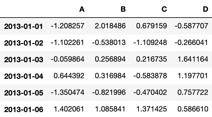
              dtype='datetime64[ns]', freq='D')

df = pd.DataFrame(np.random.randn(6, 4), index=dates, columns=list('ABCD'))
df

Output：

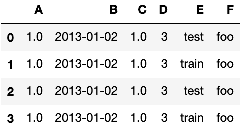
用 Series 字典对象生成 DataFrame：

df2 = pd.DataFrame({'A': 1.,
                    'B': pd.Timestamp('20130102'),
                    'C': pd.Series(1, index=list(range(4)), dtype='float32'),
                    'D': np.array([3] * 4, dtype='int32'),
                    'E': pd.Categorical(["test", "train", "test", "train"]),
                    'F': 'foo'})
df2

Output：

DataFrame 的列有不同数据类型：

df2.dtypes

# Output
A           float64
B    datetime64[ns]
C           float32
D             int32
E          category
F            object
dtype: object

IPython支持 tab 键自动补全列名与公共属性。下面是部分可自动补全的属性：

• df2.A
• df2.abs
• df2.add
• df2.add_prefix
• df2.add_suffix
• df2.align
• df2.all
• df2.any
• df2.append
• df2.apply
• df2.applymap
• df2.D
• df2.bool
• df2.boxplot
• df2.C
• df2.clip
• df2.clip_lower
• df2.clip_upper
• df2.columns
• df2.combine
• df2.combine_first
• df2.compound
• df2.consolidate

列 A、B、C、D 和 E 都可以自动补全；为简洁起见，此处只显示了部分属性。

查看数据

# 查看 DataFrame 头部数据
df.head()
# 查看 DataFrame 尾部数据
df.tail(3)
# 显示索引
df.index
# 显示列名
df.columns
# 显示值
df.values
# 快速查看数据的统计摘要
df.describe()
# 转制数据
df.T
# 按轴排序
df.sort_index(axis=1, ascending=False)
# 按值排序
df.sort_values(by='B')

获取数据

选择

提醒
选择、设置标准 Python / Numpy 的表达式已经非常直观，交互也很方便，但对于生产代码，我们还是推荐优化过的 Pandas 数据访问方法：.at、.iat、.loc 和 .iloc。

详见索引与选择数据、多层索引与高级索引文档。

# 选择单列，产生 Series，与 `df.A` 等效
df['A']

# Output
2013-01-01   -1.208257
2013-01-02   -1.102261
2013-01-03   -0.059864
2013-01-04    0.644392
2013-01-05   -1.350474
2013-01-06    1.402061
Freq: D, Name: A, dtype: float64

按标签选择

# 用标签提取一行数据
df.loc[dates[0]]

# Output
A   -1.208257
B    2.018486
C    0.679159
D   -0.587707
Name: 2013-01-01 00:00:00, dtype: float64

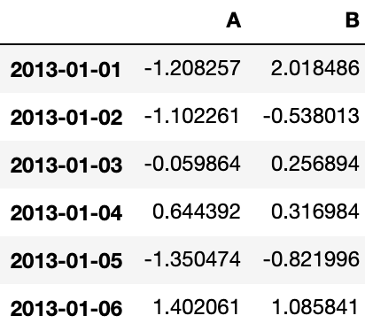
# 用标签选择多列数据
df.loc[:, ['A', 'B']]

Output：

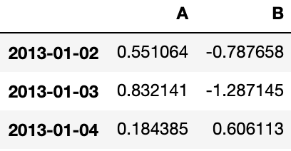
用标签切片，包含行与列结束点

df.loc['20130102':'20130104', ['A', 'B']]

Output：

# 返回对象降维
df.loc['20130102', ['A', 'B']]

# Output
A   -1.102261
B   -0.538013
Name: 2013-01-02 00:00:00, dtype: float64

# 提取标量值
df.loc[dates[0], 'A']
# Output
-1.2082567185245703

# 快速访问标量，与 loc 等效
df.at[dates[0], 'A']
# Output
-1.2082567185245703

按位置选择

用整数位置选择：

df.iloc[3]
# Output
A    0.644392
B    0.316984
C   -0.583878
D    1.197701
Name: 2013-01-04 00:00:00, dtype: float64

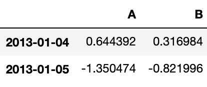
# 类似 NumPy / Python，用整数切片：
df.iloc[3:5, 0:2]

Output：

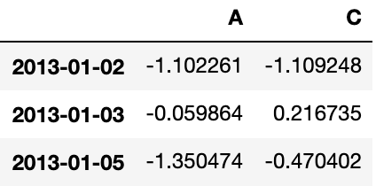
# 类似 NumPy / Python，用整数列表按位置切片：
df.iloc[[1, 2, 4], [0, 2]]

Output：

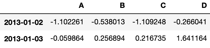
# 显式整行切片
df.iloc[1:3, :]

Output：

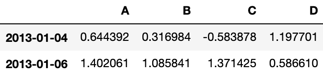
# 显式整列切片
df.iloc[:, 1:3]

Output：

# 显式提取值
df.iloc[1, 1]
# Output
-0.5380131662468983

# 快速访问标量 等效与 iloc
df.iat[1, 1]
# Output
-0.5380131662468983

布尔索引

# 用单列的值选择数据
df[df.A > 0]

Output：

# 选择 DataFrame 里满足条件的值
df[df > 0]

Output：

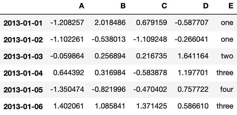
# 用 isin() 筛选
df2 = df.copy()
df2['E'] = ['one', 'one', 'two', 'three', 'four', 'three']
df2

Output：

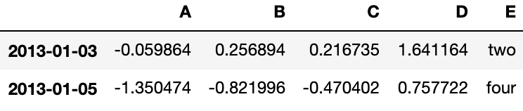
df2[df2['E'].isin(['two', 'four'])]

Output：

赋值

用索引自动对齐新增列的数据：

s1 = pd.Series([1, 2, 3, 4, 5, 6], index=pd.date_range('20130102', periods=6))
s1
# Output
2013-01-02    1
2013-01-03    2
2013-01-04    3
2013-01-05    4
2013-01-06    5
2013-01-07    6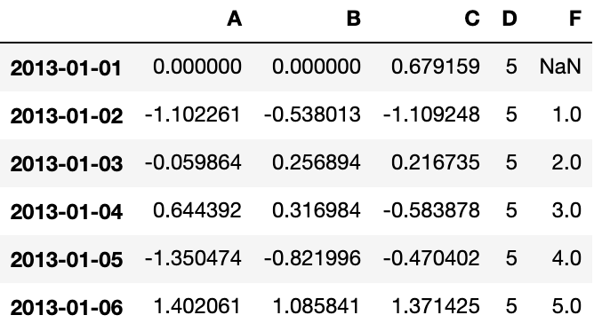
Freq: D, dtype: int64

df['F'] = s1

# 按标签赋值
df.at[dates[0], 'A'] = 0

# 按位置赋值
df.iat[0, 1] = 0

# 按 NumPy 数组赋值
df.loc[:, 'D'] = np.array([5] * len(df))

df

Output：

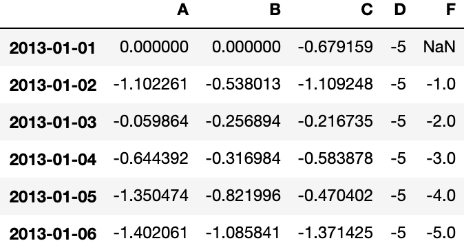
# 用 where 条件赋值
df2 = df.copy()
df2[df2 > 0] = -df2
df2

Output：

缺失值

Pandas 主要用 np.nan 表示缺失数据。 计算时，默认不包含空值。详见缺失数据。

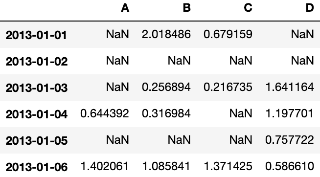
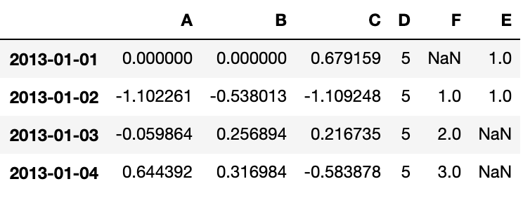
重建索引（reindex）可以更改、添加、删除指定轴的索引，并返回数据副本，即不更改原数据。

df1 = df.reindex(index=dates[0:4], columns=list(df.columns) + ['E'])
df1.loc[dates[0]:dates[1], 'E'] = 1
df1

Output：

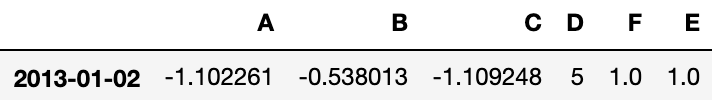
# 删除所有含缺失值的行
df1.dropna(how='any')

Output：

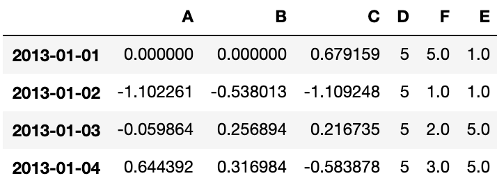
# 填充缺失值
df1.fillna(value=5)

Output：

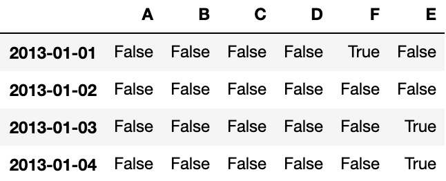
# 提取 nan 值的布尔掩码
pd.isna(df1)

运算

二进制操作

统计

一般情况下，运算时排除缺失值。
描述性统计：

df.mean()
# Output
A   -0.077691
B    0.049952
C    0.017299
D    5.000000
F    3.000000
dtype: float64

# 在另一个轴(即，行)上执行同样的操作
df.mean(1)

# Output
2013-01-01    1.419790
2013-01-02    0.650095
2013-01-03    1.482753
2013-01-04    1.675500
2013-01-05    1.271426
2013-01-06    2.771865
Freq: D, dtype: float64

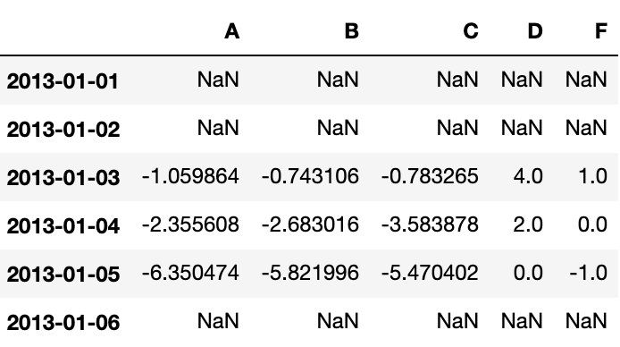
# 不同维度对象运算时，要先对齐。 此外，Pandas 自动沿指定维度广播
s = pd.Series([1, 3, 5, np.nan, 6, 8], index=dates).shift(2)
s

# Output
2013-01-01    NaN
2013-01-02    NaN
2013-01-03    1.0
2013-01-04    3.0
2013-01-05    5.0
2013-01-06    NaN
Freq: D, dtype: float64

df.sub(s, axis='index')

Apply 函数

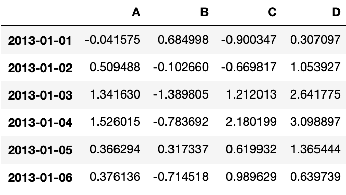
Apply 函数处理数据：

df.apply(np.cumsum)

Output：

df.apply(lambda x: x.max() - x.min())
# Output
A    2.752535
B    1.907837
C    2.480673
D    0.000000
F    4.000000
dtype: float64

直方图

s = pd.Series(np.random.randint(0, 7, size=10))
s
# Output
0    2
1    5
2    1
3    6
4    0
5    0
6    6
7    0
8    6
9    3
dtype: int64

s.value_counts()
# Output
6    3
0    3
5    1
3    1
2    1
1    1
dtype: int64

字符串方法

Series 的 str 属性包含一组字符串处理功能，如下列代码所示。注意，str 的模式匹配默认使用正则表达式。详见矢量字符串方法。

s = pd.Series(['A', 'B', 'C', 'Aaba', 'Baca', np.nan, 'CABA', 'dog', 'cat'])
s.str.lower()

# Output
0       a
1       b
2       c
3    aaba
4    baca
5     NaN
6    caba
7     dog
8     cat
dtype: object

合并（Merge）

结合（Concat）

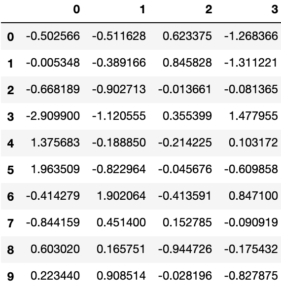
Pandas 提供了多种将 Series、DataFrame 对象组合在一起的功能，用索引与关联代数功能的多种设置逻辑可执行连接（join）与合并（merge）操作。
concat() 用于连接 Pandas 对象：

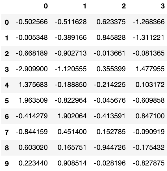
df = pd.DataFrame(np.random.randn(10, 4))
df

Output：

# 分解为多组
pieces = [df[:3], df[3:7], df[7:]]
pd.concat(pieces)

Output：

连接（join）

SQL 风格的合并。 详见数据库风格连接

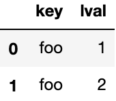
left = pd.DataFrame({'key': ['foo', 'foo'], 'lval': [1, 2]})
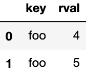
right = pd.DataFrame({'key': ['foo', 'foo'], 'rval': [4, 5]})
left

Output：

right

Output：

合并

pd.merge(left, right, on='key')

Output：

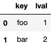
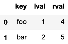
left = pd.DataFrame({'key': ['foo', 'bar'], 'lval': [1, 2]})
right = pd.DataFrame({'key': ['foo', 'bar'], 'rval': [4, 5]})
left

Output：

right

Output：

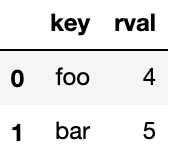
pd.merge(left, right, on='key')

Output：

追加（Append）

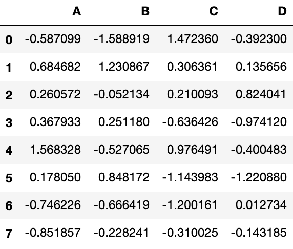
为 DataFrame 追加行。

df = pd.DataFrame(np.random.randn(8, 4), columns=['A', 'B', 'C', 'D'])
df

Output：

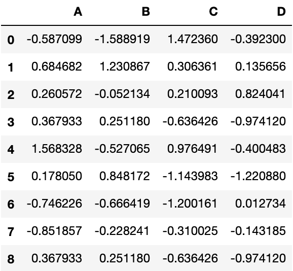
s = df.iloc[3]
df.append(s, ignore_index=True)

Output：

分组（Grouping）

“group by” 指的是涵盖下列一项或多项步骤的处理流程：

• 分割：按条件把数据分割成多组；
• 应用：为每组单独应用函数；
• 组合：将处理结果组合成一个数据结构。

  df = pd.DataFrame({'A': ['foo', 'bar', 'foo', 'bar',
                         'foo', 'bar', 'foo', 'foo'],
                   'B': ['one', 'one', 'two', 'three',
                         'two', 'two', 'one', 'three'],
                   'C': np.random.randn(8),
                   'D': np.random.randn(8)})
  df

Output：

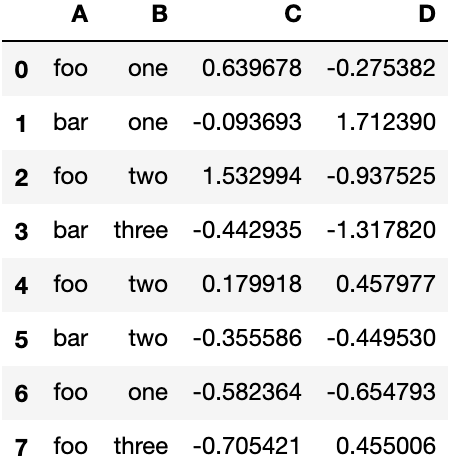
# 先分组，再用 sum()函数计算每组的汇总数据
df.groupby('A').sum()

Output：

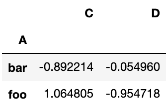
多列分组后，生成多层索引，也可以应用 sum 函数：

df.groupby(['A', 'B']).sum()

重塑（Reshaping）

详见多层索引与重塑

堆叠（Stack）

tuples = list(zip(*[['bar', 'bar', 'baz', 'baz',
                     'foo', 'foo', 'qux', 'qux'],
                    ['one', 'two', 'one', 'two',
                     'one', 'two', 'one', 'two']]))
index = pd.MultiIndex.from_tuples(tuples, names=['first', 'second'])
df = pd.DataFrame(np.random.randn(8, 2), index=index, columns=['A', 'B'])
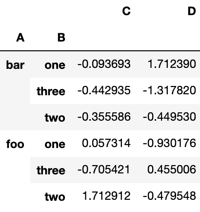
df2 = df[:4]
df2

Output：

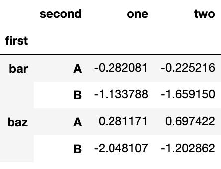
stack()方法把 DataFrame 列压缩至一层：

stacked = df2.stack()
stacked
# Output
first  second
bar    one     A   -0.282081
               B   -1.133788
       two     A   -0.225216
               B   -1.659150
baz    one     A    0.281171
               B   -2.048107
       two     A    0.697422
               B   -1.202862
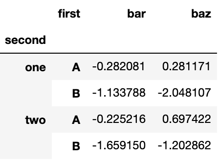
dtype: float64

压缩后的 DataFrame 或 Series 具有多层索引， stack() 的逆操作是 unstack()，默认为拆叠最后一层：

stacked.unstack()

Output：

stacked.unstack(1)

Output：

stacked.unstack(0)

Output：

数据透视表（Pivot Tables）

df = pd.DataFrame({'A': ['one', 'one', 'two', 'three'] * 3,
                   'B': ['A', 'B', 'C'] * 4,
                   'C': ['foo', 'foo', 'foo', 'bar', 'bar', 'bar'] * 2,
                   'D': np.random.randn(12),
                   'E': np.random.randn(12)})
df

Output：

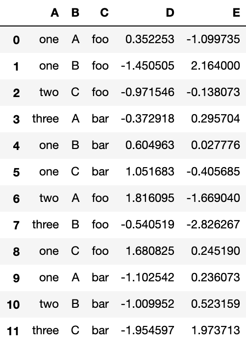
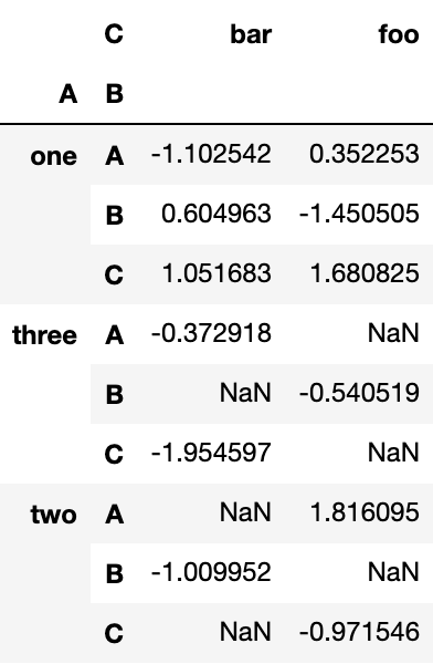
用上述数据生成数据透视表非常简单：

pd.pivot_table(df, values='D', index=['A', 'B'], columns=['C'])

Output：

时间序列(TimeSeries)

Pandas 为频率转换时重采样提供了虽然简单易用，但强大高效的功能，如，将秒级的数据转换为 5 分钟为频率的数据。这种操作常见于财务应用程序，但又不仅限于此。

rng = pd.date_range('1/1/2012', periods=100, freq='S')
ts = pd.Series(np.random.randint(0, 500, len(rng)), index=rng)
ts.resample('5Min').sum()

# Output
2012-01-01    27830
Freq: 5T, dtype: int64

# 时区表示
rng = pd.date_range('3/6/2012 00:00', periods=5, freq='D')
ts = pd.Series(np.random.randn(len(rng)), rng)
ts

# Output
2012-03-06   -0.122874
2012-03-07    3.048883
2012-03-08    0.974570
2012-03-09    0.676963
2012-03-10    1.857628
Freq: D, dtype: float64

ts_utc = ts.tz_localize('UTC')
ts_utc

# Output
2012-03-06 00:00:00+00:00   -0.122874
2012-03-07 00:00:00+00:00    3.048883
2012-03-08 00:00:00+00:00    0.974570
2012-03-09 00:00:00+00:00    0.676963
2012-03-10 00:00:00+00:00    1.857628
Freq: D, dtype: float64

# 转换成其它时区
ts_utc.tz_convert('US/Eastern')

# Output
2012-03-05 19:00:00-05:00   -0.122874
2012-03-06 19:00:00-05:00    3.048883
2012-03-07 19:00:00-05:00    0.974570
2012-03-08 19:00:00-05:00    0.676963
2012-03-09 19:00:00-05:00    1.857628
Freq: D, dtype: float64

# 转换时间段
rng = pd.date_range('1/1/2012', periods=5, freq='M')
ts = pd.Series(np.random.randn(len(rng)), index=rng)
ts

# Output
2012-01-31   -1.263639
2012-02-29   -0.101891
2012-03-31   -0.578687
2012-04-30   -1.472608
2012-05-31    0.565977
Freq: M, dtype: float64

ps = ts.to_period()
ps

# Output
2012-01   -1.263639
2012-02   -0.101891
2012-03   -0.578687
2012-04   -1.472608
2012-05    0.565977
Freq: M, dtype: float64

ps.to_timestamp()

# Output
2012-01-01   -1.263639
2012-02-01   -0.101891
2012-03-01   -0.578687
2012-04-01   -1.472608
2012-05-01    0.565977
Freq: MS, dtype: float64

Pandas 函数可以很方便地转换时间段与时间戳。下例把以 11 月为结束年份的季度频率转换为下一季度月末上午 9 点：

prng = pd.period_range('1990Q1', '2000Q4', freq='Q-NOV')
ts = pd.Series(np.random.randn(len(prng)), prng)
ts.index = (prng.asfreq('M', 'e') + 1).asfreq('H', 's') + 9
ts.head()

# Output
1990-03-01 09:00   -1.147739
1990-06-01 09:00    1.924324
1990-09-01 09:00   -0.451538
1990-12-01 09:00    0.978331
1991-03-01 09:00   -0.419933
Freq: H, dtype: float64

类别型（Categoricals）

Pandas 的 DataFrame 里可以包含类别数据。API 文档

df = pd.DataFrame({"id": [1, 2, 3, 4, 5, 6],
                   "raw_grade": ['a', 'b', 'b', 'a', 'a', 'e']})
# 将 grade 的原生数据转换为类别型数据
df["grade"] = df["raw_grade"].astype("category")
df["grade"]

# Output
0    a
1    b
2    b
3    a
4    a
5    e
Name: grade, dtype: category
Categories (3, object): [a, b, e]

用有含义的名字重命名不同类型，调用 Series.cat.categories。

df["grade"].cat.categories = ["very good", "good", "very bad"]

重新排序各类别，并添加缺失类，Series.cat 的方法默认返回新 Series。

df["grade"] = df["grade"].cat.set_categories(["very bad", "bad", "medium",
                                              "good", "very good"])
df["grade"]

# Output
0    very good
1         good
2         good
3    very good
4    very good
5     very bad
Name: grade, dtype: category
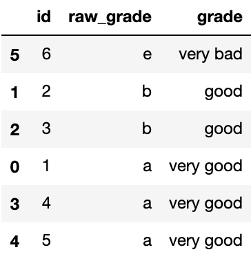
Categories (5, object): [very bad, bad, medium, good, very good]

注意，这里是按生成类别时的顺序排序，不是按词汇排序：

df.sort_values(by="grade")

Output：

按类列分组（groupby）时，即便某类别为空，也会显示：

df.groupby("grade").size()

# Output
grade
very bad     1
bad          0
medium       0
good         2
very good    3
dtype: int64

可视化

ts = pd.Series(np.random.randn(1000),
               index=pd.date_range('1/1/2000', periods=1000))
ts = ts.cumsum()
ts.plot()

Output：

<matplotlib.axes._subplots.AxesSubplot at 0x11a89e240>

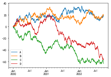
DataFrame 的 plot() 方法可以快速绘制所有带标签的列：

df = pd.DataFrame(np.random.randn(1000, 4), index=ts.index,
                  columns=['A', 'B', 'C', 'D'])
df = df.cumsum()
import matplotlib.pyplot as plt
plt.figure()
df.plot()
plt.legend(loc='best')

Output：

<matplotlib.legend.Legend at 0x11c9dc198>
<Figure size 432x288 with 0 Axes>

数据输入 / 输出

CSV

# 写入 CSV 文件
df.to_csv('foo.csv')

# 读取 CSV 文件数据
pd.read_csv('foo.csv')

HDF5

# 写入 HDF5 Store
df.to_hdf('foo.h5', 'df')

# 读取 HDF5 Store
pd.read_hdf('foo.h5', 'df')

Excel

# 写入 Excel 文件
df.to_excel('foo.xlsx', sheet_name='Sheet1')

# 读取 Excel 文件
pd.read_excel('foo.xlsx', 'Sheet1', index_col=None, na_values=['NA'])

各种坑（Gotchas）

执行某些操作，将触发异常，如：

>>> if pd.Series([False, True, False]):
...    print("I was true")

Traceback
    ...
ValueError: The truth value of an array is ambiguous. Use a.empty, a.any() or a.all().

参阅比较操作文档，查看错误提示与解决方案。详见各种坑文档。Pandas

本作品采用《CC 协议》，转载必须注明作者和本文链接