
Python 数据挖掘-如何赢得英雄联盟 LOL?游戏获胜与哪些特征更相关
0 / 1 / 创建于 5年前
 bobin123 的个人博客
简介数据集获取关注加点赞截图 加群+qq群:606115027(找管理发给你)
英雄联盟(League of Legends, LoL)是Riot Games为微软Windows和macOS开发和发行的一款多人在线战斗竞技场游戏。
在《英雄联盟》中,玩家扮演一个拥有独特能力的“冠军”角色,与一组其他玩家或电脑控制的冠军进行战斗。
游戏的目标通常是摧毁对方的“Nexus”,即一个位于由防御结构保护的基地中心的结构,尽管其他不同的游戏模式也存在着不同的目标、规则和地图。每一场《英雄联盟》的比赛都是离散的,所有的冠军一开始都相对较弱,但在游戏过程中会通过累积道具和经验来增强实力。
此数据集包含前10分钟。大约的数据,10k排名游戏(SOLO QUEUE)从高ELO (DIAMOND I to MASTER)。
玩家的级别大致相同。在游戏10分钟后,每个团队有19个特性(总共38个)。这包括死亡,死亡,黄金,经验,关卡…
这取决于你去做一些特性工程来获得更多的见解。列blueWins是目标值(我们试图预测的值)。1表示蓝队赢了。
本篇的目的是预测哪些特征与LOL获胜更相关。
设置
In [1]:
导入包和数据
import pandas as pd
import numpy as np
import matplotlib.pyplot as plt
import seaborn as sns
In [2]:
%matplotlib inline
sns.set_style(‘darkgrid’)
In [3]:
df = pd.read_csv(‘/home/kesci/input/lol8974/high_diamond_ranked_10min.csv’)
df.head()
Out[3]:
| gameId | blueWins | blueWardsPlaced | blueWardsDestroyed | blueFirstBlood | blueKills | blueDeaths | blueAssists | blueEliteMonsters | blueDragons | … | redTowersDestroyed | redTotalGold | redAvgLevel | redTotalExperience | redTotalMinionsKilled | redTotalJungleMinionsKilled | redGoldDiff | redExperienceDiff | redCSPerMin | redGoldPerMin | |
|---|---|---|---|---|---|---|---|---|---|---|---|---|---|---|---|---|---|---|---|---|---|
| 0 | 4519157822 | 0 | 28 | 2 | 1 | 9 | 6 | 11 | 0 | 0 | … | 0 | 16567 | 6.8 | 17047 | 197 | 55 | -643 | 8 | 19.7 | 1656.7 |
| 1 | 4523371949 | 0 | 12 | 1 | 0 | 5 | 5 | 5 | 0 | 0 | … | 1 | 17620 | 6.8 | 17438 | 240 | 52 | 2908 | 1173 | 24.0 | 1762.0 |
| 2 | 4521474530 | 0 | 15 | 0 | 0 | 7 | 11 | 4 | 1 | 1 | … | 0 | 17285 | 6.8 | 17254 | 203 | 28 | 1172 | 1033 | 20.3 | 1728.5 |
| 3 | 4524384067 | 0 | 43 | 1 | 0 | 4 | 5 | 5 | 1 | 0 | … | 0 | 16478 | 7.0 | 17961 | 235 | 47 | 1321 | 7 | 23.5 | 1647.8 |
| 4 | 4436033771 | 0 | 75 | 4 | 0 | 6 | 6 | 6 | 0 | 0 | … | 0 | 17404 | 7.0 | 18313 | 225 | 67 | 1004 | -230 | 22.5 | 1740.4 |
5 rows × 40 columns
EDA
In [4]:
检查缺少的值和数据类型
df.info()
<class ‘pandas.core.frame.DataFrame’>
RangeIndex: 9879 entries, 0 to 9878
Data columns (total 40 columns):
gameId 9879 non-null int64
blueWins 9879 non-null int64
blueWardsPlaced 9879 non-null int64
blueWardsDestroyed 9879 non-null int64
blueFirstBlood 9879 non-null int64
blueKills 9879 non-null int64
blueDeaths 9879 non-null int64
blueAssists 9879 non-null int64
blueEliteMonsters 9879 non-null int64
blueDragons 9879 non-null int64
blueHeralds 9879 non-null int64
blueTowersDestroyed 9879 non-null int64
blueTotalGold 9879 non-null int64
blueAvgLevel 9879 non-null float64
blueTotalExperience 9879 non-null int64
blueTotalMinionsKilled 9879 non-null int64
blueTotalJungleMinionsKilled 9879 non-null int64
blueGoldDiff 9879 non-null int64
blueExperienceDiff 9879 non-null int64
blueCSPerMin 9879 non-null float64
blueGoldPerMin 9879 non-null float64
redWardsPlaced 9879 non-null int64
redWardsDestroyed 9879 non-null int64
redFirstBlood 9879 non-null int64
redKills 9879 non-null int64
redDeaths 9879 non-null int64
redAssists 9879 non-null int64
redEliteMonsters 9879 non-null int64
redDragons 9879 non-null int64
redHeralds 9879 non-null int64
redTowersDestroyed 9879 non-null int64
redTotalGold 9879 non-null int64
redAvgLevel 9879 non-null float64
redTotalExperience 9879 non-null int64
redTotalMinionsKilled 9879 non-null int64
redTotalJungleMinionsKilled 9879 non-null int64
redGoldDiff 9879 non-null int64
redExperienceDiff 9879 non-null int64
redCSPerMin 9879 non-null float64
redGoldPerMin 9879 non-null float64
dtypes: float64(6), int64(34)
memory usage: 3.0 MB
In [5]:
df_clean = df.copy()
In [6]:
#删除一些不必要的列。例如,blueFirstblood/redfirst blood blueEliteMonster/redEliteMonster blueDeath/redKills等重复
cols = [‘gameId’, ‘redFirstBlood’, ‘redKills’, ‘redEliteMonsters’, ‘redDragons’,’redTotalMinionsKilled’,
‘redTotalJungleMinionsKilled’, ‘redGoldDiff’, ‘redExperienceDiff’, ‘redCSPerMin’, ‘redGoldPerMin’, ‘redHeralds’,
‘blueGoldDiff’, ‘blueExperienceDiff’, ‘blueCSPerMin’, ‘blueGoldPerMin’, ‘blueTotalMinionsKilled’]
df_clean = df_clean.drop(cols, axis = 1)
In [7]:
df_clean.info()
<class ‘pandas.core.frame.DataFrame’>
RangeIndex: 9879 entries, 0 to 9878
Data columns (total 23 columns):
blueWins 9879 non-null int64
blueWardsPlaced 9879 non-null int64
blueWardsDestroyed 9879 non-null int64
blueFirstBlood 9879 non-null int64
blueKills 9879 non-null int64
blueDeaths 9879 non-null int64
blueAssists 9879 non-null int64
blueEliteMonsters 9879 non-null int64
blueDragons 9879 non-null int64
blueHeralds 9879 non-null int64
blueTowersDestroyed 9879 non-null int64
blueTotalGold 9879 non-null int64
blueAvgLevel 9879 non-null float64
blueTotalExperience 9879 non-null int64
blueTotalJungleMinionsKilled 9879 non-null int64
redWardsPlaced 9879 non-null int64
redWardsDestroyed 9879 non-null int64
redDeaths 9879 non-null int64
redAssists 9879 non-null int64
redTowersDestroyed 9879 non-null int64
redTotalGold 9879 non-null int64
redAvgLevel 9879 non-null float64
redTotalExperience 9879 non-null int64
dtypes: float64(2), int64(21)
memory usage: 1.7 MB
In [8]:
接下来让我们检查blue team特征参数之间的关系
g = sns.PairGrid(data=df_clean, vars=[‘blueKills’, ‘blueAssists’, ‘blueWardsPlaced’, ‘blueTotalGold’], hue=’blueWins’, size=3, palette=’Set1’)
g.map_diag(plt.hist)
g.map_offdiag(plt.scatter)
g.add_legend();
/opt/conda/lib/python3.6/site-packages/seaborn/axisgrid.py UserWarning: The
 size paramter has been renamed to height; please update your code.
warnings.warn(UserWarning(msg))

我们可以看到变量之间有很多线性对称
In [9]:
我们可以看到很多特征是高度相关的,让我们得到相关矩阵
plt.figure(figsize=(16, 12))
sns.heatmap(df_clean.drop(‘blueWins’, axis=1).corr(), cmap=’YlGnBu’, annot=True, fmt=’.2f’, vmin=0);

In [10]:
基于相关性矩阵,让我们稍微清理一下数据集,以避免共线性
cols = [‘blueAvgLevel’, ‘redWardsPlaced’, ‘redWardsDestroyed’, ‘redDeaths’, ‘redAssists’, ‘redTowersDestroyed’,
‘redTotalExperience’, ‘redTotalGold’, ‘redAvgLevel’]
df_clean = df_clean.drop(cols, axis=1)
In [11]:
接下来让我们删除与bluewins关系不大的列
corr_list = df_clean[df_clean.columns[1:]].apply(lambda x: x.corr(df_clean[‘blueWins’]))
cols = []
for col in corr_list.index:
if (corr_list[col]>0.2 or corr_list[col]<-0.2):
cols.append(col)
cols
Out[11]:
[‘blueFirstBlood’,
‘blueKills’,
‘blueDeaths’,
‘blueAssists’,
‘blueEliteMonsters’,
‘blueDragons’,
‘blueTotalGold’,
‘blueTotalExperience’]
In [12]:
df_clean = df_clean[cols]
df_clean.head()
Out[12]:
| blueFirstBlood | blueKills | blueDeaths | blueAssists | blueEliteMonsters | blueDragons | blueTotalGold | blueTotalExperience | |
|---|---|---|---|---|---|---|---|---|
| 0 | 1 | 9 | 6 | 11 | 0 | 0 | 17210 | 17039 |
| 1 | 0 | 5 | 5 | 5 | 0 | 0 | 14712 | 16265 |
| 2 | 0 | 7 | 11 | 4 | 1 | 1 | 16113 | 16221 |
| 3 | 0 | 4 | 5 | 5 | 1 | 0 | 15157 | 17954 |
| 4 | 0 | 6 | 6 | 6 | 0 | 0 | 16400 | 18543 |
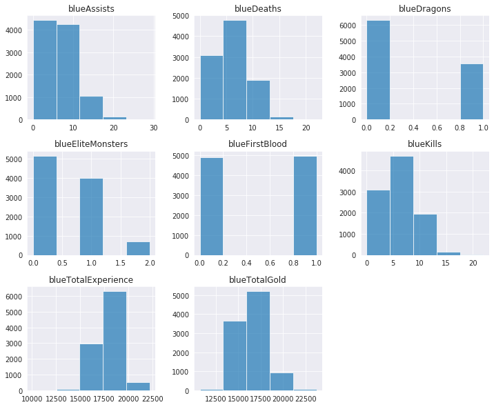
In [13]:
df_clean.hist(alpha = 0.7, figsize=(12,10), bins=5);
模型选择
In [14]:
from sklearn.preprocessing import MinMaxScaler
from sklearn.model_selection import train_test_split
X = df_clean
y = df[‘blueWins’]
scaler = MinMaxScaler()
scaler.fit(X)
X = scaler.transform(X)
X_train, X_test, y_train, y_test = train_test_split(X, y, test_size=0.2, random_state=42)
朴素贝叶斯
In [15]:
from sklearn.naive_bayes import GaussianNB
from sklearn.metrics import accuracy_score
拟合模型
clf_nb = GaussianNB()
clf_nb.fit(X_train, y_train)
pred_nb = clf_nb.predict(X_test)
得到准确性分数
acc_nb = accuracy_score(pred_nb, y_test)
print(acc_nb)
0.7176113360323887
决策树
In [16]:
拟合决策树模型
from sklearn import tree
from sklearn.model_selection import GridSearchCV
tree = tree.DecisionTreeClassifier()
搜索最好的参数
grid = {‘min_samples_split’: [5, 10, 20, 50, 100]},
clf_tree = GridSearchCV(tree, grid, cv=5)
clf_tree.fit(X_train, y_train)
pred_tree = clf_tree.predict(X_test)
获得准确度分数
acc_tree = accuracy_score(pred_tree, y_test)
print(acc_tree)
0.6928137651821862
随机森林
In [17]:
拟合模型
from sklearn.ensemble import RandomForestClassifier
rf = RandomForestClassifier()
搜索最好的参数
grid = {‘n_estimators’:[100,200,300,400,500], ‘max_depth’: [2, 5, 10]}
clf_rf = GridSearchCV(rf, grid, cv=5)
clf_rf.fit(X_train, y_train)
pred_rf = clf_rf.predict(X_test)
获得准确分数
acc_rf = accuracy_score(pred_rf, y_test)
print(acc_rf)
0.7282388663967612
逻辑回归
In [18]:
拟合逻辑回归模型
from sklearn.linear_model import LogisticRegression
lm = LogisticRegression()
lm.fit(X_train, y_train)
得到准确分数
pred_lm = lm.predict(X_test)
acc_lm = accuracy_score(pred_lm, y_test)
print(acc_lm)
0.7302631578947368
/opt/conda/lib/python3.6/site-packages/sklearn/linear_model/logistic.py FutureWarning: Default solver will be changed to ‘lbfgs’ in 0.22. Specify a solver to silence this warning.
FutureWarning)
K-近邻算法(KNN)
In [19]:
拟合模型
from sklearn.neighbors import KNeighborsClassifier
knn = KNeighborsClassifier()
搜索最好的参数
grid = {“n_neighbors”:np.arange(1,100)}
clf_knn = GridSearchCV(knn, grid, cv=5)
clf_knn.fit(X_train,y_train)
得到准确分数
pred_knn = clf_knn.predict(X_test)
acc_knn = accuracy_score(pred_knn, y_test)
print(acc_knn)
0.7171052631578947
结论
In [20]:
data_dict = {‘Naive Bayes’: [acc_nb], ‘DT’: [acc_tree], ‘Random Forest’: [acc_rf], ‘Logistic Regression’: [acc_lm], ‘K_nearest Neighbors’: [acc_knn]}
df_c = pd.DataFrame.from_dict(data_dict, orient=’index’, columns=[‘Accuracy Score’])
print(df_c)
Accuracy ScoreNaive Bayes 0.717611
DT 0.692814
Random Forest 0.728239
Logistic Regression 0.730263
K_nearest Neighbors 0.717105
从精度分数可以看出,逻辑回归和随机森林的预测效果最好。接下来让我们仔细看看这两种方法的召回率和精确率
In [21]:
召回率和精确率
from sklearn.metrics import recall_score, precision_score
lm参数
recall_lm = recall_score(pred_lm, y_test, average = None)
precision_lm = precision_score(pred_lm, y_test, average = None)
print(‘precision score for naive bayes: {}\n recall score for naive bayes:{}’.format(precision_lm, recall_lm))
precision score for naive bayes: [0.72736521 0.73313192]
recall score for naive bayes:[0.72959184 0.73092369]
In [22]:
rf参数
recall_rf = recall_score(pred_rf, y_test, average = None)
precision_rf = precision_score(pred_rf, y_test, average = None)
print(‘precision score for naive bayes: {}\n recall score for naive bayes:{}’.format(precision_rf, recall_rf))
precision score for naive bayes: [0.73550356 0.72104733]
recall score for naive bayes:[0.723 0.73360656]
一般情况下,还是会选择逻辑回归
In [23]:
df_clean.columns
Out[23]:
Index([‘blueFirstBlood’, ‘blueKills’, ‘blueDeaths’, ‘blueAssists’,
‘blueEliteMonsters’, ‘blueDragons’, ‘blueTotalGold’,
‘blueTotalExperience’],
dtype=’object’)
In [24]:
lm.coef_
Out[24]:
array([[ 0.09223084, 1.6863957 , -4.9521688 , -0.28960539, 0.30701029,
0.29102466, 5.33422084, 1.55350489]])
In [25]:
np.exp(lm.coef_)
Out[25]:
array([[1.09661794e+00, 5.39998244e+00, 7.06806308e-03, 7.48558900e-01,
1.35935495e+00, 1.33779758e+00, 2.07311157e+02, 4.72801236e+00]])
In [26]:
coef_data = np.concatenate((lm.coef_, np.exp(lm.coef_)),axis=0)
coef_df = pd.DataFrame(data=coef_data, columns=df_clean.columns).T.reset_index().rename(columns={‘index’: ‘Var’, 0: ‘coef’, 1: ‘oddRatio’})
coef_df.sort_values(by=’coef’, ascending=False)
Out[26]:
| Var | coef | oddRatio | |
|---|---|---|---|
| 6 | blueTotalGold | 5.334221 | 207.311157 |
| 1 | blueKills | 1.686396 | 5.399982 |
| 7 | blueTotalExperience | 1.553505 | 4.728012 |
| 4 | blueEliteMonsters | 0.307010 | 1.359355 |
| 5 | blueDragons | 0.291025 | 1.337798 |
| 0 | blueFirstBlood | 0.092231 | 1.096618 |
| 3 | blueAssists | -0.289605 | 0.748559 |
| 2 | blueDeaths | -4.952169 | 0.007068 |
PCA
In [27]:
使用PCA让结果可视化
X = df_clean
y = df[‘blueWins’]
PCA受scale的影响,首先要对数据集进行scale
from sklearn import preprocessing
S标准化特征
X = preprocessing.StandardScaler().fit_transform(X)
In [28]:
from sklearn.decomposition import PCA
pca = PCA(n_components=2)
components = pca.fit_transform(X)
print(pca.explained_variance_ratio_)
[0.42435947 0.20805752]
In [29]:
创造可视化df
df_vis = pd.DataFrame(data = components, columns = [‘pc1’, ‘pc2’])
df_vis = pd.concat([df_vis, df[‘blueWins’]], axis = 1)
X = df_vis[[‘pc1’, ‘pc2’]]
y = df_vis[‘blueWins’]
X_train, X_test, y_train, y_test = train_test_split(X, y, test_size=0.2, random_state=42)
In [30]:
重新定义pca数据
lm.fit(X_train, y_train)
/opt/conda/lib/python3.6/site-packages/sklearn/linear_model/logistic.py FutureWarning: Default solver will be changed to ‘lbfgs’ in 0.22. Specify a solver to silence this warning.
FutureWarning)
Out[30]:
LogisticRegression(C=1.0, class_weight=None, dual=False, fit_intercept=True,
intercept_scaling=1, l1_ratio=None, max_iter=100,
multi_class=’warn’, n_jobs=None, penalty=’l2’,
random_state=None, solver=’warn’, tol=0.0001, verbose=0,
warm_start=False)
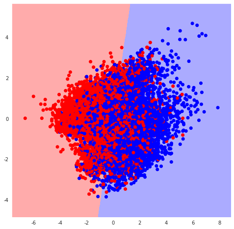
In [31]:
可视化函数
from matplotlib.colors import ListedColormap
def DecisionBoundary(clf):
X = df_vis[[‘pc1’, ‘pc2’]]
y = df_vis[‘blueWins’]
h = .02

# 创建颜色映射
cmap_light = ListedColormap(['#FFAAAA', '#AAAAFF'])
cmap_bold = ListedColormap(['#FF0000', '#0000FF'])

# 绘制决策边界。为此,我们将为每一个分配一个颜色
# 网格 [x_min, x_max]x[y_min, y_max].
x_min, x_max = X.iloc[:, 0].min() - 1, X.iloc[:, 0].max() + 1
y_min, y_max = X.iloc[:, 1].min() - 1, X.iloc[:, 1].max() + 1
xx, yy = np.meshgrid(np.arange(x_min, x_max, h),
                     np.arange(y_min, y_max, h))
Z = clf.predict(np.c_[xx.ravel(), yy.ravel()])
Z = Z.reshape(xx.shape)
plt.figure(figsize=(8, 8))
plt.pcolormesh(xx, yy, Z, cmap=cmap_light)

# Plot also the training points
plt.scatter(X.iloc[:, 0], X.iloc[:, 1], c=y, cmap=cmap_bold)
plt.xlim(xx.min(), xx.max())
plt.ylim(yy.min(), yy.max())
plt.show()
In [32]:
DecisionBoundary(lm)
本作品采用《CC 协议》,转载必须注明作者和本文链接


 关于 LearnKu


推荐文章: