在复现 GitHub 上的 SMT_Tutorial 项目时，2D 图片能够正常生成，但 3D 图片在复现时出现了点数畸形，并且呈现竖条状分布。请问这可能是什么原因，如何解决这个问题？
from future import print_function, division
import numpy as np
from scipy import linalg
from smt.utils.misc import compute_rms_error

from smt.problems import Sphere, NdimRobotArm, Rosenbrock
from smt.sampling_methods import LHS
from smt.surrogate_models import LS, QP, KPLS, KRG, KPLSK, GEKPLS, MGP

#to ignore warning messages
import warnings
warnings.filterwarnings(“ignore”)

try:
from smt.surrogate_models import IDW, RBF, RMTC, RMTB
compiled_available = True
except:
compiled_available = False

try:
import matplotlib.pyplot as plt
plot_status = True
except:
plot_status = False

import scipy.interpolate

from mpl_toolkits.mplot3d import Axes3D
import matplotlib.pyplot as plt
from matplotlib import cm

########### Initialization of the problem, construction of the training and validation points

ndim = 2
ndoe = 20 #int(10*ndim)

Define the function

fun = Rosenbrock(ndim=ndim)

Construction of the DOE

in order to have the always same LHS points, random_state=1

sampling = LHS(xlimits=fun.xlimits, criterion=’ese’, random_state=1)
xt = sampling(ndoe)

Compute the outputs

yt = fun(xt)

Construction of the validation points

ntest = 200 #500
sampling = LHS(xlimits=fun.xlimits, criterion=’ese’, random_state=1)
xtest = sampling(ntest)
ytest = fun(xtest)

#To visualize the DOE points
fig = plt.figure(figsize=(10, 10))
plt.scatter(xt[:,0],xt[:,1],marker = ‘x’,c=’b’,s=200,label=’Training points’)
plt.scatter(xtest[:,0],xtest[:,1],marker = ‘.’,c=’k’, s=200, label=’Validation points’)
plt.title(‘DOE’)
plt.xlabel(‘x1’)
plt.ylabel(‘x2’)
plt.legend()
plt.show()

To plot the Rosenbrock function

x = np.linspace(-2,2,50)
res = []
for x0 in x:
for x1 in x:
res.append(fun(np.array([[x0,x1]])))
res = np.array(res)
res = res.reshape((50,50)).T
X,Y = np.meshgrid(x,x)
fig = plt.figure(figsize=(15, 10))
ax = fig.add_subplot(projection=’3d’)
surf = ax.plot_surface(X, Y, res, cmap=cm.viridis,
linewidth=0, antialiased=False,alpha=0.5)

ax.scatter(xt[:,0],xt[:,1],yt,zdir=’z’,marker = ‘x’,c=’b’,s=200,label=’Training point’)
ax.scatter(xtest[:,0],xtest[:,1],ytest,zdir=’z’,marker = ‘.’,c=’k’,s=200,label=’Validation point’)

plt.title(‘Rosenbrock function’)
plt.xlabel(‘x1’)
plt.ylabel(‘x2’)
plt.legend()
plt.show()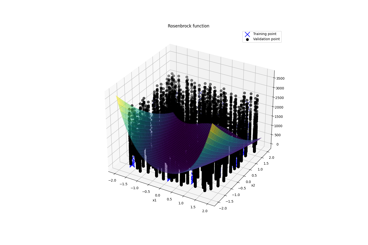

图1 复现代码畸形图片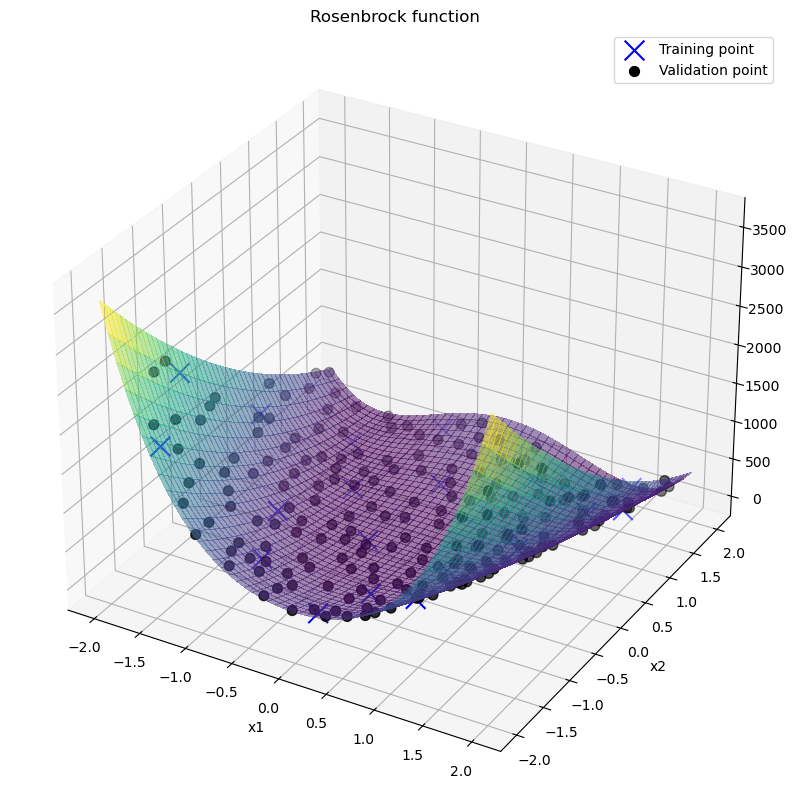

图2 项目作者生成图片

项目链接：github.com/SMTorg/smt/blob/master/...